Graphviz and mermaid in DiagrammeR • DiagrammeR

Graphviz

Graphviz support is an integral part of the DiagrammeR package. Graphviz consists of a graph description language called the DOT language and it also comprises various tools that can process the DOT language. DOT is highly customizable and it allows you to control line colors, arrow shapes, node shapes, and many other layout features.

DiagrammeR Implementation

For Graphviz graphs, DiagrammeR uses the processing function called grViz(). What you pass into grViz() is a valid graph specification in the DOT language. The DOT graph description can either be delivered to grViz() in the form of a string, a reference to a Graphviz file (with a .gv file extension), or as a text connection.

All of the code examples provided in later sections call the grViz() function in an R script and pass in a graph description as a string. It is important to consider that strings in R cannot contain any unescaped double-quote characters. However, the grViz() function allows for single-quote characters in their place. As a further convenience, when the DOT graph description is supplied as a file (e.g., dot-graph.gv) or as a text connection, either format for quotes will be accepted.

In very recent builds of RStudio, the use of an external text file with the .gv file extension can provide the advantage of syntax coloring and previewing in the RStudio Viewer pane after saving (if 'Preview on Save' is selected), or, by pressing the 'Preview' button on the Source pane.

Defining a Graphviz Graph

The Graphviz graph specification must begin with a directive stating whether a directed graph (digraph) or an undirected graph (graph) is desired. Semantically, this indicates whether or not there is a natural direction from one of the edge’s nodes to the other. An optional graph ID follows this and paired curly braces denotes the body of the statement list (stmt_list).

Optionally, a graph may also be described as strict. This forbids the creation of multi-edges (i.e., there can be at most one edge with a given tail node and head node in the directed case). For undirected graphs, there can be at most one edge connected to the same two nodes. Subsequent edge statements using the same two nodes will identify the edge with the previously defined one and apply any attributes given in the edge statement.

Here is the basic structure:

[strict] (graph | digraph) [ID] '{' stmt_list '}'

Statements

The graph statement (graph_stmt), the node statement (node_stmt), and the edge statement (edge_stmt) are the three most commonly used statements in the Graphviz DOT language. Graph statements allow for attributes to be set for all components of the graph. Node statements define and provide attributes for graph nodes. Edge statements specify the edge operations between nodes and they supply attributes to the edges. For the edge operations, a directed graph must specify an edge using the edge operator -> while an undirected graph must use the -- operator.

Within these statements follow statement lists. Thus for a node statement, a list of nodes is expected. For an edge statement, a list of edge operations. Any of the list items can optionally have an attribute list (attr_list) which modify the attributes of either the node or edge.

Comments may be placed within the statement list. These can be marked using a // or a /* */ structure. Comment lines are denoted by a # character. Multiple statements within a statement list can be separated by linebreaks or ; characters between multiple statements

Here is an example where nodes (in this case styled as boxes and circles) can be easily defined along with their connections:

grViz("
digraph boxes_and_circles {

  # a 'graph' statement
  graph [overlap = true, fontsize = 10]

  # several 'node' statements
  node [shape = box,
        fontname = Helvetica]
  A; B; C; D; E; F

  node [shape = circle,
        fixedsize = true,
        width = 0.9] // sets as circles
  1; 2; 3; 4; 5; 6; 7; 8

  # several 'edge' statements
  A->1 B->2 B->3 B->4 C->A
  1->D E->A 2->4 1->5 1->F
  E->6 4->6 5->7 6->7 3->8
}
")

Subgraphs and Clusters

Subgraphs play three roles in Graphviz. First, a subgraph can be used to represent graph structure, indicating that certain nodes and edges should be grouped together. This is the usual role for subgraphs and typically specifies semantic information about the graph components. It can also provide a convenient shorthand for edges. An edge statement allows a subgraph on both the left and right sides of the edge operator. When this occurs, an edge is created from every node on the left to every node on the right. For example, the specification

A -> {B C}

is equivalent to

A -> B
A -> C

In the second role, a subgraph can provide a context for setting attributes. For example, a subgraph could specify that blue is the default color for all nodes defined in it. In the context of graph drawing, a more interesting example is

subgraph {
  rank = same; A; B; C;
}

This anonymous subgraph specifies that the nodes A, B, and C should all be placed on the same rank.

The third role for subgraphs directly involves how the graph will be laid out by certain layout types. If the name of the subgraph begins with cluster, Graphviz notes the subgraph as a special cluster subgraph. If supported, the layout will make it such that the nodes belonging to the cluster are drawn together, with the entire drawing of the cluster contained within a bounding rectangle.

Graphviz Attributes

Graphviz attributes allow you to style your Graphviz graph. Combinations of attributes for nodes, edges, clusters, and for the entire graph provide for highly-customized layouts.

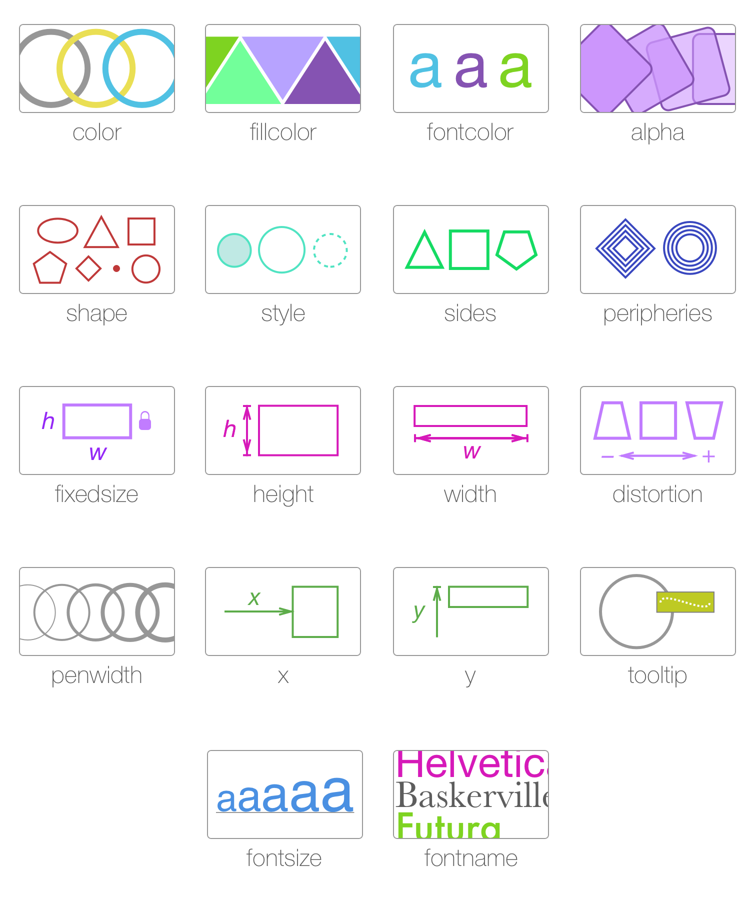
Node Attributes

All Graphviz attributes are specified by name-value pairs. Thus, to set the fillcolor of a node abc, one would use

abc [fillcolor = red]

There are lots of node attributes. The following provides a visual guide to the more notable ones.

X11 Colors

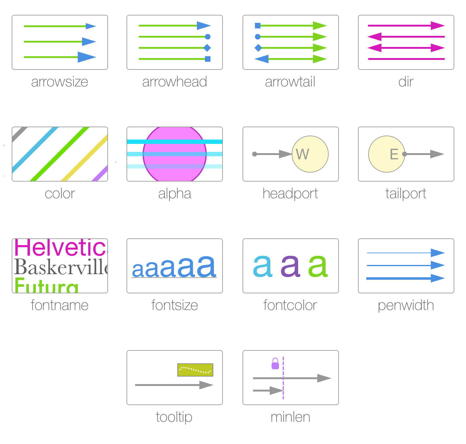
Edge Attributes

Edge attributes are set the same way as node attributes. For example, to set the arrowhead style of an edge abc -> def, one would use

abc -> def [arrowhead = diamond]

Quotation marks are important only for multiword attributes, such might be used in the label attribute.

Refer to the following for some of the more important edge attributes

X11 Colors

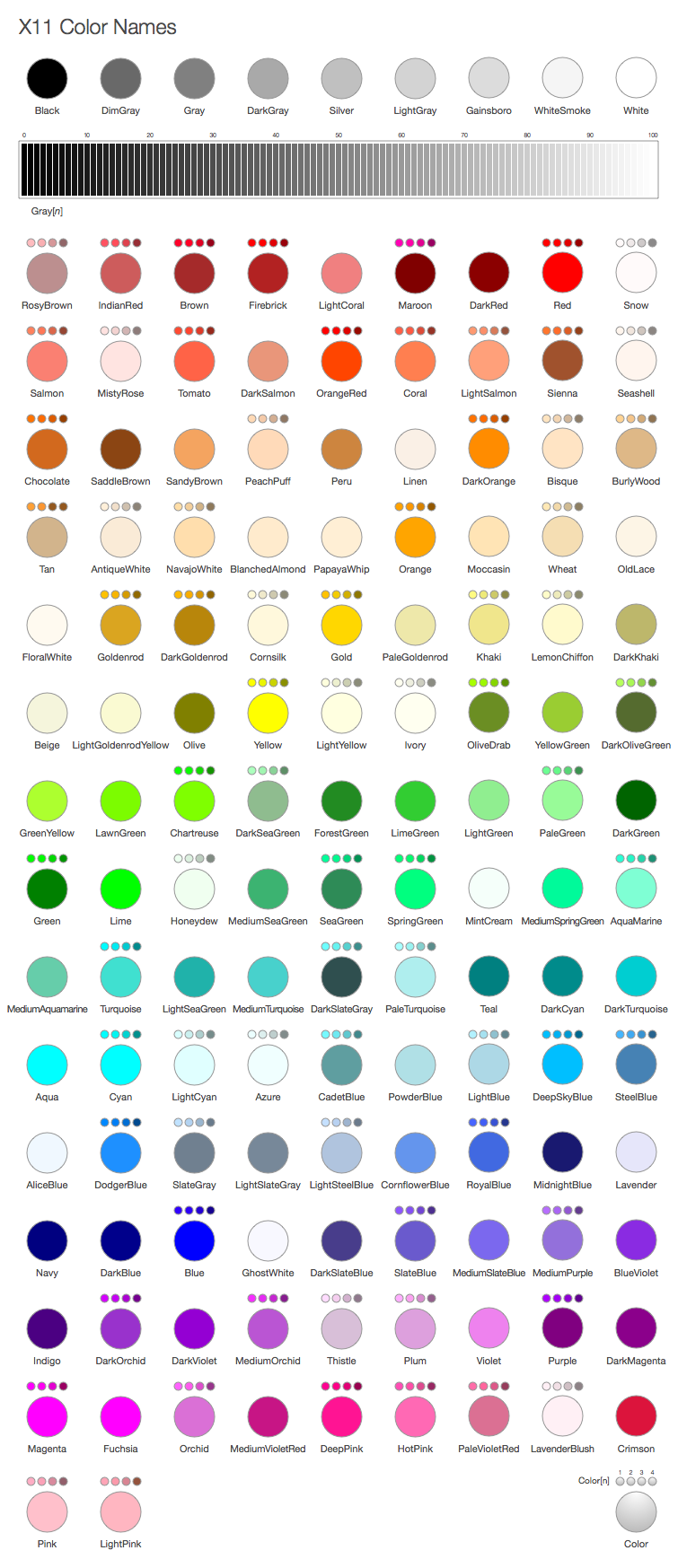
Colors

By default, Graphviz can use colors provided as hexadecimal values, or, as X11 color names. The following provides the entire list of X11 color names. Some colors have additional 4-color palettes based on the named color. Those additional colors can be used by appending the digits 1-4 to the color name. Gray (or grey) has variations from 0-100. Please note that, in all color names, gray is interchangeable with grey.

X11 Colors

Node Shapes

There’s no shortage of shapes available for nodes. Nodes can be changed from the default ellipse shape by using the shape parameter. This table provides a listing of all the possible node shapes.

Arrow Shapes

The shapes of arrows are highly customizable. When defining an edge, the arrowhead parameter allows you change the style of arrowhead from the default normal arrow shape, to one of several others. Here are some of the other arrowhead types that could be used.

Graphviz Substitution

Graphviz substitution allows for mixing in R expressions into a Graphviz DOT graph specification without sacrificing readability.

How It Works

To take advantage of substitution when rendering a graph, simply use the grViz() function with Graphviz DOT code:

grViz("
[...graph spec with substitutions using @@ notation and footnote R expressions...]
")

The notation @@ within the GraphViz DOT graph specification will indicate where the substitution is to take place. Corresponding R expressions (below the formal graph specification, styled as footnotes) will provide values to be substituted. The grViz() function will autodetect whether the working Graphviz DOT graph specification contains @@s between the curly braces of the [graph|digraph] {...} DOT construction.

If you specify a substitution with @@, you must ensure there is a valid expression for that substitution. The expressions are placed as footnotes and their evaluations must result in an R vector object (i.e., not a data frame, list, or matrix). Because there is the possibility to have multiple substitutions, numbering is required. Thus, the @@ notation is immediately followed by a number and that number should correspond to the number of the footnoted R expression.

The substitution construction is:

"@@" + [footnote number]

Importantly, the footnote expressions should reside below the closing curly brace of the graph or digraph expression. It should always take the form of:

"[" + [footnote number] + "]:"

In the simple example of specifying a single node, the following substitution syntax would be used:

digraph {
@@1
}

[1]: 'a'

In the above example, the [1]: footnote expression evaluates as 'a', and, that is what’s substituted in place of the @@1 (the resultant a, in turn, will be taken as the node ID).

Substitutions can also be used to insert values from vector indices into the graph specification. Simply use this format:

"@@" + [footnote number] + "-" + [index number]

Here’s an example of how specific values from vectors can be inserted into the graph:

digraph alpha {
  
  @@1-1; @@1-2; @@1-3; @@1-4; @@1-5
  @@1-6; @@1-7; @@1-8; @@1-9; @@1-10
}

[1]: LETTERS

After evaluation of the footnote expressions and substitution, the graph specification becomes this:

digraph alpha {
  
  A; B; C; D; E
  F; G; H; I; J
}

Examples

The best way to demonstrate how substitution works is through a set of examples. Here is an example of substituting alphabet letters from R’s LETTERS constant into a Graphviz graph specification.

You can mix substitutions of single-values objects and those specifying indices of R vector objects. As an example:

grViz("
digraph a_nice_graph {

# node definitions with substituted label text
node [fontname = Helvetica]
a [label = '@@1']
b [label = '@@2-1']
c [label = '@@2-2']
d [label = '@@2-3']
e [label = '@@2-4']
f [label = '@@2-5']
g [label = '@@2-6']
h [label = '@@2-7']
i [label = '@@2-8']
j [label = '@@2-9']

# edge definitions with the node IDs
a -> {b c d e f g h i j}
}

[1]: 'top'
[2]: 10:20
")

As can be seen from the output:

the node with ID a is given the label “top” (after substituting @@1 with expression after the [1]: footnote R expression)
the nodes with ID values from b to j are respectively provided values from indices 1 to 9 (using the hyphenated form of @@) of the evaluated expression 10:20 (in the [2]: footnote expression)

Footnote expressions are meant to be flexible. They can span multiple lines, and they can also take in objects that are available in the global workspace. So, as long as a vector object results from evaluation, substitution can be performed.