# Visualizing survival

A survival curve is far easier to understand as a picture than as a table of numbers. By default Greenwood draws curves with [Altair](https://altair-viz.github.io/), which produces interactive charts (tooltips and zoom) and is Narwhals-native: the numbers flow straight from your Polars fit into the chart with no Pandas or Matplotlib in the way, so a pure Polars/Narwhals workflow stays pure. This page covers the survival curve plot, confidence bands, censoring marks, and the numbers-at-risk table. A [plotnine](https://plotnine.org/) backend, for a grammar-of-graphics workflow, is described near the end.

Altair is an optional dependency. If you installed Greenwood with the `altair` extra, or with `all`, you already have it. We use the `lung` dataset throughout. First we build the response.


``` python
import greenwood as gw

lung = gw.load_dataset("lung", backend="polars")

y = gw.Surv.right(lung["time"], event=(lung["status"] == 2))
y
```


    Surv(type=right, n=228, events=165)


We then fit a Kaplan-Meier estimator stratified by sex, one curve per group, using the log-log confidence interval transform. Printing the fitted estimator summarizes each stratum.


``` python
km = gw.KaplanMeier(conf_type="log-log").fit(y, by=lung["sex"])
km
```


    KaplanMeier (Kaplan-Meier survival estimate)

         n  events  median  0.95LCL  0.95UCL
    1  138     112     270      210      306
    2   90      53     426      345      524


Everything below draws from this fitted `km` object. Before plotting, it also helps to see the numbers the curve is built from. Calling [to_frame()](../reference/AFT.md#greenwood.AFT.to_frame) on the fitted estimator returns the step-function estimates in tidy form, one row per stratum and time, with the survival probability and its confidence limits. The preview shows the first and last rows along with the full dimensions of the table.


``` python
km.to_frame(format="polars")
```


<table class="gt_table" data-quarto-disable-processing="true" data-quarto-bootstrap="false">
<thead>
<tr class="gt_heading">
<th colspan="10" class="gt_heading gt_title gt_font_normal"><div style="padding-top: 0; padding-bottom: 7px;">
<span class="gd-tbl-badge" style="background-color: #0075FF; color: #FFFFFF; border: 1px solid #0075FF; margin-right: 8px;">Polars</span>Rows206Columns9
</div></th>
</tr>
<tr class="gt_col_headings">
<th class="gt_col_heading gt_columns_bottom_border gt_right" scope="col"></th>
<th id="strata" class="gt_col_heading gt_columns_bottom_border gt_left" scope="col"><div>

strata

<em>obj</em>

</div></th>
<th id="time" class="gt_col_heading gt_columns_bottom_border gt_right" scope="col"><div>

time

<em>f64</em>

</div></th>
<th id="n_risk" class="gt_col_heading gt_columns_bottom_border gt_right" scope="col"><div>

n_risk

<em>f64</em>

</div></th>
<th id="n_event" class="gt_col_heading gt_columns_bottom_border gt_right" scope="col"><div>

n_event

<em>f64</em>

</div></th>
<th id="n_censor" class="gt_col_heading gt_columns_bottom_border gt_right" scope="col"><div>

n_censor

<em>f64</em>

</div></th>
<th id="estimate" class="gt_col_heading gt_columns_bottom_border gt_right" scope="col"><div>

estimate

<em>f64</em>

</div></th>
<th id="std_error" class="gt_col_heading gt_columns_bottom_border gt_right" scope="col"><div>

std_error

<em>f64</em>

</div></th>
<th id="conf_low" class="gt_col_heading gt_columns_bottom_border gt_right" scope="col"><div>

conf_low

<em>f64</em>

</div></th>
<th id="conf_high" class="gt_col_heading gt_columns_bottom_border gt_right" scope="col"><div>

conf_high

<em>f64</em>

</div></th>
</tr>
</thead>
<tbody class="gt_table_body">
<tr>
<td class="gt_row gt_right gd-tbl-rownum">0</td>
<td class="gt_row gt_left" style="max-width: 63px">1</td>
<td class="gt_row gt_right" style="max-width: 50px">11</td>
<td class="gt_row gt_right" style="max-width: 63px">138</td>
<td class="gt_row gt_right" style="max-width: 71px">3</td>
<td class="gt_row gt_right" style="max-width: 78px">0</td>
<td class="gt_row gt_right" style="max-width: 124px">0.978260869565</td>
<td class="gt_row gt_right" style="max-width: 124px">0.0124139182765</td>
<td class="gt_row gt_right" style="max-width: 124px">0.934121582525</td>
<td class="gt_row gt_right" style="max-width: 117px">0.992936557511</td>
</tr>
<tr>
<td class="gt_row gt_right gd-tbl-rownum">1</td>
<td class="gt_row gt_left" style="max-width: 63px">1</td>
<td class="gt_row gt_right" style="max-width: 50px">12</td>
<td class="gt_row gt_right" style="max-width: 63px">135</td>
<td class="gt_row gt_right" style="max-width: 71px">1</td>
<td class="gt_row gt_right" style="max-width: 78px">0</td>
<td class="gt_row gt_right" style="max-width: 124px">0.971014492754</td>
<td class="gt_row gt_right" style="max-width: 124px">0.014281169221</td>
<td class="gt_row gt_right" style="max-width: 124px">0.924619139392</td>
<td class="gt_row gt_right" style="max-width: 117px">0.989021541626</td>
</tr>
<tr>
<td class="gt_row gt_right gd-tbl-rownum">2</td>
<td class="gt_row gt_left" style="max-width: 63px">1</td>
<td class="gt_row gt_right" style="max-width: 50px">13</td>
<td class="gt_row gt_right" style="max-width: 63px">134</td>
<td class="gt_row gt_right" style="max-width: 71px">2</td>
<td class="gt_row gt_right" style="max-width: 78px">0</td>
<td class="gt_row gt_right" style="max-width: 124px">0.95652173913</td>
<td class="gt_row gt_right" style="max-width: 124px">0.0173597697718</td>
<td class="gt_row gt_right" style="max-width: 124px">0.905787300104</td>
<td class="gt_row gt_right" style="max-width: 117px">0.980228948021</td>
</tr>
<tr>
<td class="gt_row gt_right gd-tbl-rownum">3</td>
<td class="gt_row gt_left" style="max-width: 63px">1</td>
<td class="gt_row gt_right" style="max-width: 50px">15</td>
<td class="gt_row gt_right" style="max-width: 63px">132</td>
<td class="gt_row gt_right" style="max-width: 71px">1</td>
<td class="gt_row gt_right" style="max-width: 78px">0</td>
<td class="gt_row gt_right" style="max-width: 124px">0.949275362319</td>
<td class="gt_row gt_right" style="max-width: 124px">0.0186795340253</td>
<td class="gt_row gt_right" style="max-width: 124px">0.896548509216</td>
<td class="gt_row gt_right" style="max-width: 117px">0.975490402087</td>
</tr>
<tr>
<td class="gt_row gt_right gd-tbl-rownum">4</td>
<td class="gt_row gt_left" style="max-width: 63px">1</td>
<td class="gt_row gt_right" style="max-width: 50px">26</td>
<td class="gt_row gt_right" style="max-width: 63px">131</td>
<td class="gt_row gt_right" style="max-width: 71px">1</td>
<td class="gt_row gt_right" style="max-width: 78px">0</td>
<td class="gt_row gt_right" style="max-width: 124px">0.942028985507</td>
<td class="gt_row gt_right" style="max-width: 124px">0.019892897278</td>
<td class="gt_row gt_right" style="max-width: 124px">0.887428391293</td>
<td class="gt_row gt_right" style="max-width: 117px">0.970579101988</td>
</tr>
<tr>
<td class="gt_row gt_right gd-tbl-rownum">5</td>
<td class="gt_row gt_left" style="max-width: 63px">1</td>
<td class="gt_row gt_right" style="max-width: 50px">30</td>
<td class="gt_row gt_right" style="max-width: 63px">130</td>
<td class="gt_row gt_right" style="max-width: 71px">1</td>
<td class="gt_row gt_right" style="max-width: 78px">0</td>
<td class="gt_row gt_right" style="max-width: 124px">0.934782608696</td>
<td class="gt_row gt_right" style="max-width: 124px">0.0210182948563</td>
<td class="gt_row gt_right" style="max-width: 124px">0.878418312188</td>
<td class="gt_row gt_right" style="max-width: 117px">0.965522040145</td>
</tr>
<tr>
<td class="gt_row gt_right gd-tbl-rownum">6</td>
<td class="gt_row gt_left" style="max-width: 63px">1</td>
<td class="gt_row gt_right" style="max-width: 50px">31</td>
<td class="gt_row gt_right" style="max-width: 63px">129</td>
<td class="gt_row gt_right" style="max-width: 71px">1</td>
<td class="gt_row gt_right" style="max-width: 78px">0</td>
<td class="gt_row gt_right" style="max-width: 124px">0.927536231884</td>
<td class="gt_row gt_right" style="max-width: 124px">0.0220691880472</td>
<td class="gt_row gt_right" style="max-width: 124px">0.869508906988</td>
<td class="gt_row gt_right" style="max-width: 117px">0.960339509261</td>
</tr>
<tr class="gd-tbl-divider">
<td class="gt_row gt_right gd-tbl-rownum">7</td>
<td class="gt_row gt_left" style="max-width: 63px">1</td>
<td class="gt_row gt_right" style="max-width: 50px">53</td>
<td class="gt_row gt_right" style="max-width: 63px">128</td>
<td class="gt_row gt_right" style="max-width: 71px">2</td>
<td class="gt_row gt_right" style="max-width: 78px">0</td>
<td class="gt_row gt_right" style="max-width: 124px">0.913043478261</td>
<td class="gt_row gt_right" style="max-width: 124px">0.0239859688855</td>
<td class="gt_row gt_right" style="max-width: 124px">0.851957778533</td>
<td class="gt_row gt_right" style="max-width: 117px">0.949657700321</td>
</tr>
<tr>
<td class="gt_row gt_right gd-tbl-rownum">203</td>
<td class="gt_row gt_left" style="max-width: 63px">2</td>
<td class="gt_row gt_right" style="max-width: 50px">765</td>
<td class="gt_row gt_right" style="max-width: 63px">3</td>
<td class="gt_row gt_right" style="max-width: 71px">1</td>
<td class="gt_row gt_right" style="max-width: 78px">0</td>
<td class="gt_row gt_right" style="max-width: 124px">0.0832144435134</td>
<td class="gt_row gt_right" style="max-width: 124px">0.0499212744378</td>
<td class="gt_row gt_right" style="max-width: 124px">0.0185052512122</td>
<td class="gt_row gt_right" style="max-width: 117px">0.212363854832</td>
</tr>
<tr>
<td class="gt_row gt_right gd-tbl-rownum">204</td>
<td class="gt_row gt_left" style="max-width: 63px">2</td>
<td class="gt_row gt_right" style="max-width: 50px">821</td>
<td class="gt_row gt_right" style="max-width: 63px">2</td>
<td class="gt_row gt_right" style="max-width: 71px">0</td>
<td class="gt_row gt_right" style="max-width: 78px">1</td>
<td class="gt_row gt_right" style="max-width: 124px">0.0832144435134</td>
<td class="gt_row gt_right" style="max-width: 124px">0.0499212744378</td>
<td class="gt_row gt_right" style="max-width: 124px">0.0185052512122</td>
<td class="gt_row gt_right" style="max-width: 117px">0.212363854832</td>
</tr>
<tr>
<td class="gt_row gt_right gd-tbl-rownum">205</td>
<td class="gt_row gt_left" style="max-width: 63px">2</td>
<td class="gt_row gt_right" style="max-width: 50px">965</td>
<td class="gt_row gt_right" style="max-width: 63px">1</td>
<td class="gt_row gt_right" style="max-width: 71px">0</td>
<td class="gt_row gt_right" style="max-width: 78px">1</td>
<td class="gt_row gt_right" style="max-width: 124px">0.0832144435134</td>
<td class="gt_row gt_right" style="max-width: 124px">0.0499212744378</td>
<td class="gt_row gt_right" style="max-width: 124px">0.0185052512122</td>
<td class="gt_row gt_right" style="max-width: 117px">0.212363854832</td>
</tr>
</tbody>
</table>


Each row is a step in one of the curves. The `time` and `estimate` columns give the point at which the survival probability drops and its value after the drop, while `conf_low` and `conf_high` give the band that the plot will shade. The `strata` column identifies the group, so there is one set of steps per sex, and `n_risk`, `n_event`, and `n_censor` record how many subjects were at risk, failed, or were censored at each time. The plot turns exactly these numbers into a picture.


# The survival curve plot

The main entry point is [plot_survival](../reference/plot_survival.md#greenwood.plot_survival). Given a fitted [KaplanMeier](../reference/KaplanMeier.md#greenwood.KaplanMeier), it draws the step curve for each stratum, a shaded confidence band, and a small notch at each censoring time.


``` python
lung = gw.load_dataset("lung", backend="polars")

y = gw.Surv.right(lung["time"], event=(lung["status"] == 2))
km = gw.KaplanMeier(conf_type="log-log").fit(y, by=lung["sex"])

gw.plot_survival(km)
```


Each element carries meaning. The steps show the estimated survival probability, the band shows its uncertainty, and the censoring notches -- angled so they sit on the curve without obscuring it -- show where subjects left the risk set without an event. Because the chart is interactive, you can hover a curve to read the survival probability at a time, and drag or scroll to zoom. Curves that separate and stay apart suggest a real group difference, which you would confirm with a log-rank test from [Comparing groups](comparing-groups.md).

You can turn individual elements off. Removing the band and the censoring marks produces a cleaner curve for a slide or a small figure.


``` python
gw.plot_survival(km, conf_int=False, censor_marks=False)
```


# Adding a numbers-at-risk table

A survival plot is much easier to trust when it is accompanied by the number of subjects still at risk at regular intervals. As the risk set shrinks, the curve becomes less certain, and the table makes that visible. Pass `risk_table=True` to stack an aligned table beneath the curve.


``` python
gw.plot_survival(km, risk_table=True)
```


The table shares the horizontal axis with the curve above it, so the counts line up with the times they describe -- and because they share one x scale, panning or zooming the curve moves the table with it. You control the times shown with the `times` argument.


``` python
gw.plot_survival(km, risk_table=True, times=[0, 250, 500, 750, 1000])
```


If you only need the numbers, `risk_table_data` returns them as a tidy frame, which you can render however you like, including through Great Tables. It is backend-neutral, so it works whether or not you have a plotting library installed.


``` python
gw.viz.risk_table_data(km, times=[0, 250, 500, 750, 1000], format="polars")
```


<table class="gt_table" data-quarto-disable-processing="true" data-quarto-bootstrap="false">
<thead>
<tr class="gt_heading">
<th colspan="4" class="gt_heading gt_title gt_font_normal"><div style="padding-top: 0; padding-bottom: 7px;">
<span class="gd-tbl-badge" style="background-color: #0075FF; color: #FFFFFF; border: 1px solid #0075FF; margin-right: 8px;">Polars</span>Rows10Columns3
</div></th>
</tr>
<tr class="gt_col_headings">
<th class="gt_col_heading gt_columns_bottom_border gt_right" scope="col"></th>
<th id="strata" class="gt_col_heading gt_columns_bottom_border gt_left" scope="col"><div>

strata

<em>str</em>

</div></th>
<th id="time" class="gt_col_heading gt_columns_bottom_border gt_right" scope="col"><div>

time

<em>f64</em>

</div></th>
<th id="n_risk" class="gt_col_heading gt_columns_bottom_border gt_right" scope="col"><div>

n_risk

<em>f64</em>

</div></th>
</tr>
</thead>
<tbody class="gt_table_body">
<tr>
<td class="gt_row gt_right gd-tbl-rownum">0</td>
<td class="gt_row gt_left" style="max-width: 159px">1</td>
<td class="gt_row gt_right" style="max-width: 146px">0</td>
<td class="gt_row gt_right" style="max-width: 159px">138</td>
</tr>
<tr>
<td class="gt_row gt_right gd-tbl-rownum">1</td>
<td class="gt_row gt_left" style="max-width: 159px">1</td>
<td class="gt_row gt_right" style="max-width: 146px">250</td>
<td class="gt_row gt_right" style="max-width: 159px">62</td>
</tr>
<tr>
<td class="gt_row gt_right gd-tbl-rownum">2</td>
<td class="gt_row gt_left" style="max-width: 159px">1</td>
<td class="gt_row gt_right" style="max-width: 146px">500</td>
<td class="gt_row gt_right" style="max-width: 159px">20</td>
</tr>
<tr>
<td class="gt_row gt_right gd-tbl-rownum">3</td>
<td class="gt_row gt_left" style="max-width: 159px">1</td>
<td class="gt_row gt_right" style="max-width: 146px">750</td>
<td class="gt_row gt_right" style="max-width: 159px">7</td>
</tr>
<tr>
<td class="gt_row gt_right gd-tbl-rownum">4</td>
<td class="gt_row gt_left" style="max-width: 159px">1</td>
<td class="gt_row gt_right" style="max-width: 146px">1000</td>
<td class="gt_row gt_right" style="max-width: 159px">2</td>
</tr>
<tr>
<td class="gt_row gt_right gd-tbl-rownum">5</td>
<td class="gt_row gt_left" style="max-width: 159px">2</td>
<td class="gt_row gt_right" style="max-width: 146px">0</td>
<td class="gt_row gt_right" style="max-width: 159px">90</td>
</tr>
<tr>
<td class="gt_row gt_right gd-tbl-rownum">6</td>
<td class="gt_row gt_left" style="max-width: 159px">2</td>
<td class="gt_row gt_right" style="max-width: 146px">250</td>
<td class="gt_row gt_right" style="max-width: 159px">53</td>
</tr>
<tr>
<td class="gt_row gt_right gd-tbl-rownum">7</td>
<td class="gt_row gt_left" style="max-width: 159px">2</td>
<td class="gt_row gt_right" style="max-width: 146px">500</td>
<td class="gt_row gt_right" style="max-width: 159px">21</td>
</tr>
<tr>
<td class="gt_row gt_right gd-tbl-rownum">8</td>
<td class="gt_row gt_left" style="max-width: 159px">2</td>
<td class="gt_row gt_right" style="max-width: 146px">750</td>
<td class="gt_row gt_right" style="max-width: 159px">3</td>
</tr>
<tr>
<td class="gt_row gt_right gd-tbl-rownum">9</td>
<td class="gt_row gt_left" style="max-width: 159px">2</td>
<td class="gt_row gt_right" style="max-width: 146px">1000</td>
<td class="gt_row gt_right" style="max-width: 159px">0</td>
</tr>
</tbody>
</table>


To draw just the aligned table as its own chart, without a curve above it, use [risk_table](../reference/risk_table.md#greenwood.risk_table).


``` python
gw.risk_table(km, times=[0, 250, 500, 750, 1000])
```


# Customizing the plot

[plot_survival](../reference/plot_survival.md#greenwood.plot_survival) returns an ordinary Altair chart, so you refine it with Altair's API. Chaining `.properties` sets the title and dimensions, and you can keep layering or restyling from there.


``` python
gw.plot_survival(km).properties(
    title="Survival by sex", width=640, height=360
)
```


> **Note: The plot is a chart object, not an image**
>
> [plot_survival](../reference/plot_survival.md#greenwood.plot_survival) returns an Altair chart (an `alt.LayerChart`, or an `alt.VConcatChart` when `risk_table=True`). It renders interactively in notebooks and browsers, and you keep composing it with Altair's API. Nothing about the figure is locked down.

> **Tip: Saving figures**
>
> Call `save` on the returned chart. Use `chart.save("survival.html")` for the interactive version, or `chart.save("survival.png")` (also `.svg`, `.pdf`) for a static image -- static export uses `vl-convert`, which ships with the `altair` extra.


# The plotnine backend

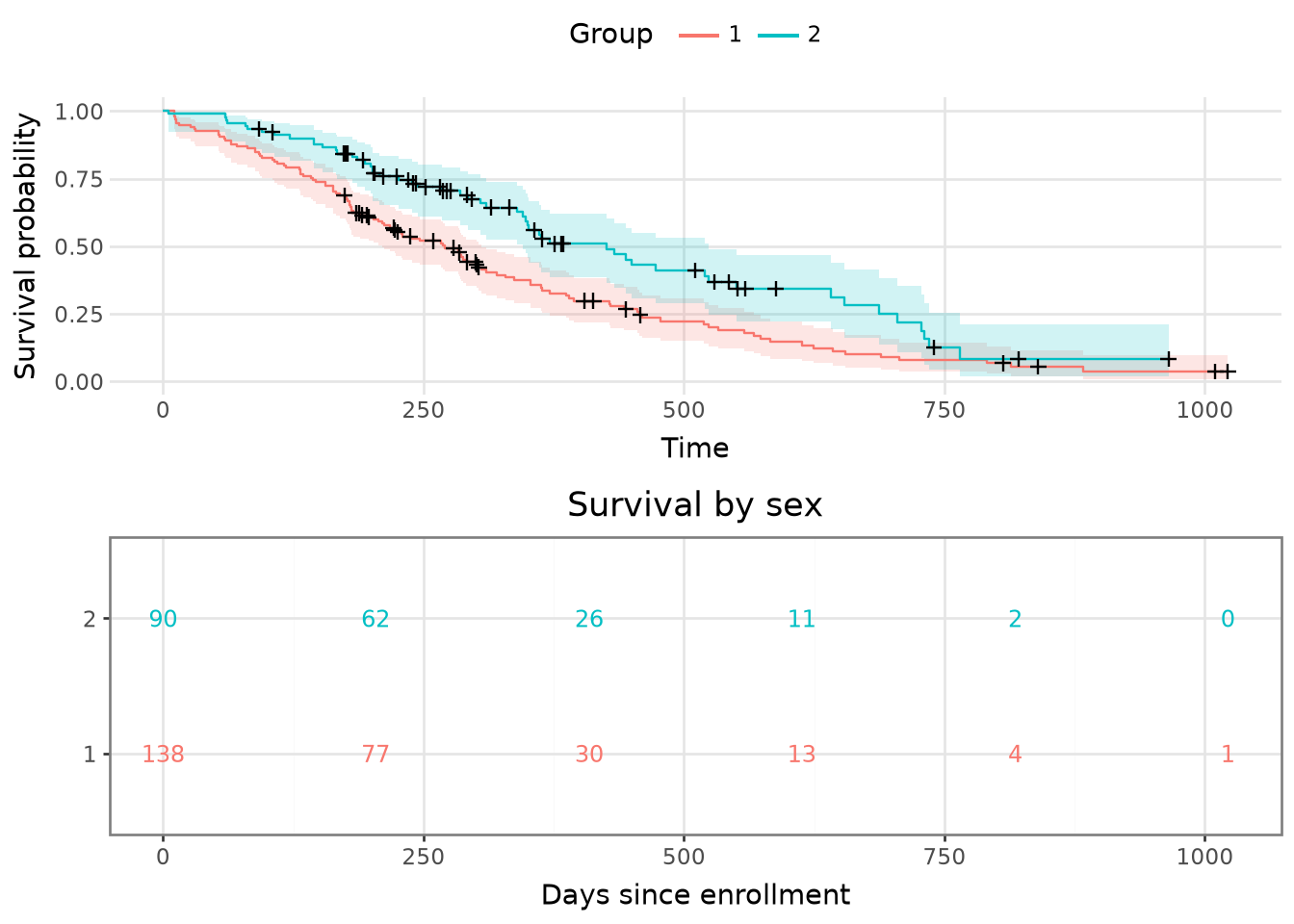
If you prefer a grammar-of-graphics workflow, or you already build figures with ggplot2-style layers, Greenwood also draws the same curves with [plotnine](https://plotnine.org/) under `greenwood.viz.plotnine`. It is an optional dependency, installed with the `plotnine` extra (or with `all`). The plotnine backend is built on Matplotlib and Pandas, so it is not part of a Pandas-free workflow, but it produces static, publication-ready figures you compose with the `+` operator.

The API mirrors the default one: [plot_survival](../reference/plot_survival.md#greenwood.plot_survival) takes the same fitted [KaplanMeier](../reference/KaplanMeier.md#greenwood.KaplanMeier) and the same `conf_int`, `censor_marks`, [risk_table](../reference/risk_table.md#greenwood.risk_table), and `times` arguments, but returns a plotnine `ggplot` (or a plotnine composition when `risk_table=True`).


``` python
from plotnine import labs, theme_bw

(
    gw.viz.plotnine.plot_survival(km, risk_table=True)
    + theme_bw()
    + labs(title="Survival by sex", x="Days since enrollment", color="Sex")
)
```


<figure class="figure">
<p><img src="visualization_files/figure-html/cell-13-output-1.png" class="figure-img" width="672" height="480" /></p>
</figure>


Because the result is a plotnine object, you extend it with any plotnine layer, scale, or theme, and you save it with its `save` method, for example `plot.save("survival.png", width=8, height=6, dpi=300)`.


# Next steps

You can now produce and customize publication-quality survival figures.

- [Cox regression](cox-regression.md) introduces models whose coefficients you will later visualize as forest plots.
- [Competing risks](competing-risks.md) produces cumulative incidence curves, which are plotted the same way.
- Revisit [Comparing groups](comparing-groups.md) to pair a grouped figure with a formal test.