# plot_schoenfeld()


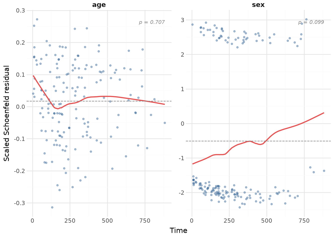
Scaled Schoenfeld residual plots for assessing proportional hazards.


Usage

``` python
plot_schoenfeld(
    cox,
    *,
    transform="identity",
    show_zph=True,
    title=None,
    backend="altair",
    width=280,
    height=200,
)
```


Plots scaled Schoenfeld residuals against event time, one panel per covariate, with a loess smooth line and a dashed reference line at the overall coefficient estimate. Under proportional hazards, the smooth should be approximately flat. A trend indicates that the covariate's effect changes over time.

This is the visual equivalent of R's `plot(cox.zph(fit))`.


## Parameters


`cox: Any`  
A fitted [CoxPH](CoxPH.md#greenwood.CoxPH) model.

`transform: str = ``"identity"`  
Time-axis transformation: `"identity"` (default), `"log"`, `"km"` (Kaplan-Meier failure probability), or `"rank"`.

`show_zph: bool = ``True`  
If `True` (default), annotate each panel with the Grambsch-Therneau test p-value from [cox_zph()](CoxPH.md#greenwood.CoxPH.cox_zph).

`title: str | None = None`  
Optional supertitle for the combined chart.

`backend: Literal[``"altair", `<span class="st">`"plotnine"``]`</span>` = ``"altair"`  
Plotting backend: `"altair"` (default) or `"plotnine"`.

`width: int = ``280`  
Width of each panel in pixels (Altair) or approximate inches × 72 (plotnine).

`height: int = ``200`  
Height of each panel in pixels (Altair) or approximate inches × 72 (plotnine).


## Returns


`alt.Chart or plotnine.ggplot`  
A composite chart (Altair `HConcatChart`) or a faceted plotnine plot.


## Examples


``` python
import greenwood as gw

lung = gw.load_dataset("lung", backend="polars")
cox = gw.CoxPH().fit("Surv(time, status) ~ age + sex", data=lung)

gw.plot_schoenfeld(cox)
```


<style>
  #altair-viz-e2cf1fe89feb404d8d302ea456b0aa47.vega-embed {
    width: 100%;
    display: flex;
  }

  #altair-viz-e2cf1fe89feb404d8d302ea456b0aa47.vega-embed details,
  #altair-viz-e2cf1fe89feb404d8d302ea456b0aa47.vega-embed details summary {
    position: relative;
  }
</style>


Use a log time axis and suppress the p-value annotation:


``` python
gw.plot_schoenfeld(cox, transform="log", show_zph=False)
```


<style>
  #altair-viz-aee59b40eafc4df080b68455378f098e.vega-embed {
    width: 100%;
    display: flex;
  }

  #altair-viz-aee59b40eafc4df080b68455378f098e.vega-embed details,
  #altair-viz-aee59b40eafc4df080b68455378f098e.vega-embed details summary {
    position: relative;
  }
</style>


Use the plotnine backend for a static ggplot object:


``` python
gw.plot_schoenfeld(cox, backend="plotnine")
```


<figure class="figure">
<p><img src="plot_schoenfeld_files/figure-html/cell-4-output-1.png" class="figure-img" width="672" height="480" /></p>
</figure>